Unsupervised Semantics: Text Class Inference

Written as a Tech Note for World Food Programme Analytics Hub

Introduction

In media analysis and marketing, it is crucial to be aware of the public perception of one’s product, company, reputation, and all other similar aspects. The format in which all those are communicated is almost always textual and mostly on social media. This brings some sort of urgency to the task of analyzing and identifying sentiment in text data. In this technote, we will be discussing a method of completely unsupervised sentiment analysis that brings you some summary of what similar texts are saying. What does unsupervised mean? It means that you have no labels to your text, which is the case most of the time. Imagine that you have thousands of customer reviews speaking of your product or thousands of social media posts expressing their opinion on your company’s work environment or anything else of this sort. Now, how can you make sense of what is going on in there when you have no idea what they are saying?

Semantic Retention: BERT Embedding

For any text to be processed, it has to be embedded.  What does text embedding mean, it means that text is transformed into a numerical vector representing it in relation to other text bodies depending on the content of each of the available text bodies. As this explanation implies, embedding is a transformation and that is exactly what the models that do this are called: Transformers. What do transformers do exactly, though?

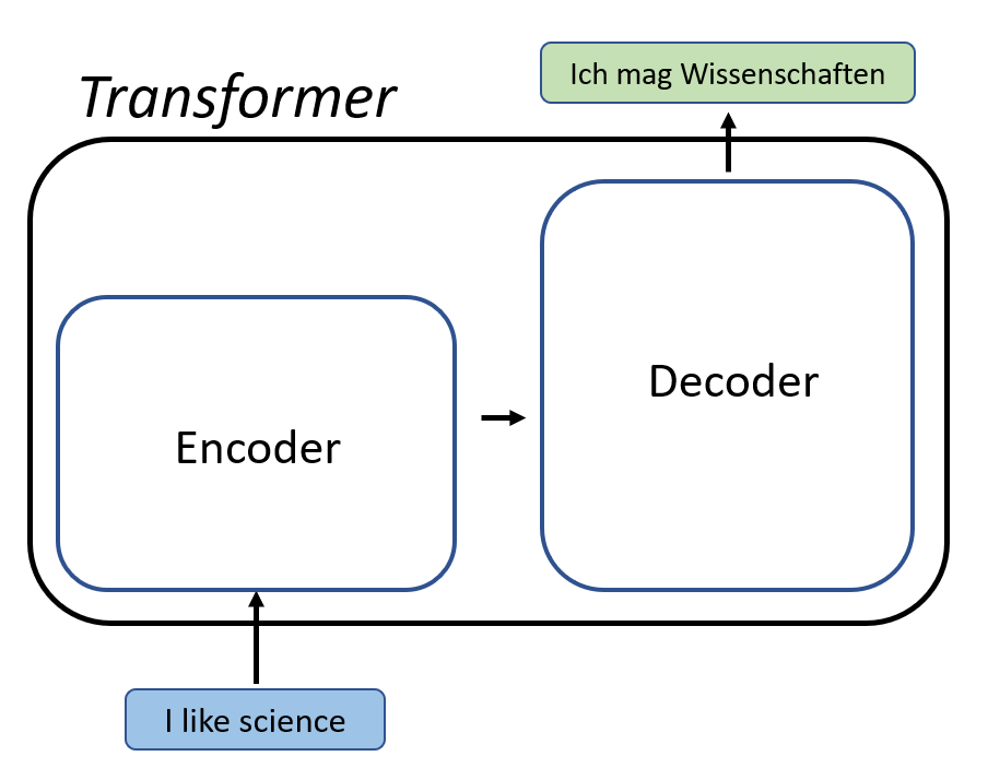
A transformer consists of two processes: Encoding and Decoding. Encoding relies on attention. In general attention is a vector of weights that captures the relationships between words and in that way capturing contexts. Given that some words correlate with others (i.e. they generally are more likely to come together) together they provide the computer with a certain kind of understanding of the context and hence meaning of the text. One might ask: how do you find the attention that best fits a certain input? The answer would be deep feedforward neural networks. Aside from the technical details of exactly how exactly an encoder works, one should just keep in mind that an encoder aims through attention and deep learning at finding a fixed-size vector that best represents the input. One of the most popular encoder models is BERT, which stands for Bidirectional Encoder Representations from Transformers. This was the model that we used for the semantic embedding of the text input, specifically we used this BERT model.

Dimensionality Reduction

If you ask yourself what is the purpose of representation, you will find out that representation is for the purpose of plotting similarity and difference at the end of the day. The metric that measures similarity and difference is the variance. So the embedding, being a 384-dimensional vector in the case of the BERT model we used, is in essence a numerical representation of the variance between whatever is represented by these numbers. What if we could have a smaller vector that can represent as much variance as the large vector? That would be great because this would require lower computational power for later processing. This is the purpose of the Principal Component Analysis (PCA)!

PCA, in a nutshell, calculates the projections of data points on the eigenvectors (i.e. components) of a certain numerical dataset, which all together explain 100% of the variance in the data. In the animation above, this is the first component and the projections of the data points on it. This is the component with the maximum variance between the projections. The second component would be the axis perpendicular on it. In the case of the above animation there are only two principal components because the number of components is equal to the minimum between number of data points and the number of dimensions. However, the first eigenvalue itself represents a lot of the variance in data, the second more than the third, third more than the fourth and so on. So, using just a couple of columns/components one could get the same results if we used the 384 dimensions. For example, check out the below graph where we used the first PCAs of an embedding of some sample text.

Similar texts are close to each other, and different ones are away from each other only using 2 columns, each one being the projections of the data points we have on the corresponding eigenvector. If we clustered them based on just two components we will get the exact same result if we clustered them using the 384 components, which is fascinating and speaks of the quality of the embedding itself.

Clustering and Internal Evaluation

Now given that the goal of embedding is representing similarity and difference, the next step is to identify both of them in an unsupervised way. This is the job of clustering. However, there are many types of clustering such as: K-Means, Hierarchical clustering, Spectral CLustering, and more. Spectral clustering was chosen for this task given its strong mathematical basis as it is based on the concept of the spectral decomposition of matrices. To avoid getting into the mathematical details of spectral clustering, the figures below demonstrate its capabilities:

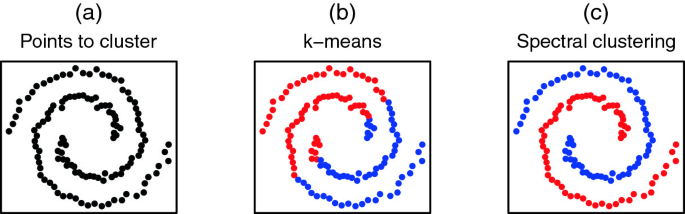
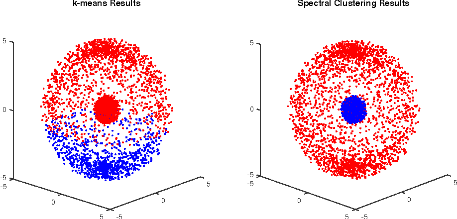
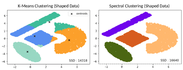
So, for our purposes the scenarios shown above (i.e. concentric or non-circular distributions of clusters) is very much likely to happen so spectral clustering should be able to cluster them correctly. But our main problem is that we have no idea about what or how the data should be labeled or which are similar to which. This means that we need to infer the best number of clusters from the embedding itself, and in this way this pipeline is completely automated and unsupervised. Internal validation in clustering relies on scores that showcase how well clustering into k clusters group data into compact clusters and separable ones. So the two most important internal validation aspects is the minimization of within-cluster distances and maximizing inter-cluster distances. A score which takes account of both aspects is the silhouette score as shown below:

The number of clusters which maximizes the silhouette score is inferred to be the best number of clusters.

A Sneak Peak into the Clusters

Now that we have performed the semantic grouping, we have clusters of data which are semantically close to each other. Here we have freedom to decide what to do with them. But this decision is up to you, and this technote aims at semantic grouping, opening the door for later processing. There are two options for providing insight into what the clusters contain: keyword extractors and summary generators.

For keyword extraction there are many options that do this.To be specific, keyword extraction is basically a derivative of NER or Named Entity Recognition. NER is the process of identifying entities in a text body and classifying according to their semantic and grammatical function such as: verbs, nouns, names, etc. The two models used for NER in this pipeline are a distilled version of BERT trained on OpenKP (is a large-scale, open-domain keyphrase extraction dataset with 148,124 real-world web documents along with 1-3 most relevant human-annotated keyphrases). DistilBERT is basically a lighter and faster version of BERT based on the same transformer architecture of BERT. The other option is to use spaCy (an open-source python library for advanced NLP tasks) to extract keywords from the combined text body of the clusters.

For summarization we used BART, which is a model developed by Facebook based on BERT-like encoder architecture with a GPT-like decoder. Decoding is basically the opposite of encoding where instead of representing text as encoders do, the representation is brought back into text using attention and feed forward neural networks to find the best way to decode as well as the architecture below shows:

This specific BART model is used in Huggingface’s summarization pipeline to provide summaries. Now the pipeline is completed theoretically, and the doors are open for later analytics in each cluster. This is because the result of this pipeline is essentially a semantic analysis of any text-based data that will provide insights into what is said in this data generally.

Testing the pipeline

For visualizing the potential of this pipeline we used ChatGPT to simulate two sets of tweets. The first set contains three sets of tweets:

1. Tweets discussing love

2. Tweets discussing the newly released Dodge RAM truck

3. Tweets discussing the rivalry between Messi and Ronaldo

The tweets are embedded, the embedding is dimensionally reduced, the embedding is clustered based on the best number of clusters inferred from the maximum silhouette score, the clustering is visualized with the first two components of the dimensionality reduction, then each cluster is combined into one text body. Finally,  each text body has keywords extracted from it using: DistilBERT and spaCy, and each text body is summarized using BART. In this specific example, best number of clusters is 3 and the clusters are shown below:

As shown above, if only those two components were used (i.e. PC1 and PC2) the clustering assignment would be correct. As obvious, the pipeline found the best clustering given that this set of tweets was divided into three topics. Now we can have the keywords extracted and the summary generated. Below are the results:

Model	1st Class	2nd Class	3rd Class
DistilBERT	'dodge' 'dodge ram'	-	'love'
spaCy	'The new Dodge Ram' 'a beast'	'The Ronaldo-Messi rivalry' 'the stuff'	'Love' 'a haunting shadow'

spaCy did a better job on this testing set, however, keyword extraction is not really enough for getting insight into the clusters. Thus, we use BART’s summarization as shown below:

class	BART Summarization
1st	The new Dodge Ram is not just a truck; it's a statement. The Dodge Ram delivers on both style and substance, a testament to its commitment to excellence. With its towing capacity and durability, the new DodgeRam is your reliable partner for any task. Experience the roar of power under the hood and the luxury within with the Dodge Ram's latest model.
2nd	The Ronaldo-Messi rivalry is the stuff of legends, a tale of two football giants who continue to redefine greatness. Every match between Ronaldo and Messi feels like a clash of titans, a spectacle that fans around the world eagerly await. The Ronaldo- Messi debate is not just about goals and assists; it's about witnessing two footballing maestros creating history.
3rd	Love is not just a feeling; it's a lifeline that connects souls. When love unravels, it can leave behind a trail of shattered dreams. Love is a journey, and each step is an exploration of the heart. The love that once made you whole can become the cause of your brokenness.

The next testing set is WFP specific “Fictional tweets”, where we have three sets of topics:

1. Tweets applauding WFP’s efforts in Afghanistan

2. Tweets saying that WFP needs to do more work in Palestine because what is done now is not enough

3. Tweets discussing what the FAO does generally

The pipeline is implemented and the best number of clusters is still correct: 3. The plot of the clusters based on the first two principal components is as follows:

The extracted keywords are as follows:

Model	1st Class	2nd Class	3rd Class
DistilBERT	'palestine' 'world food programme'	'fao' 'the fao'	'afghanistan' 'world food programme'
spaCy	'The World Food Programme's efforts' 'Palestine'	'a world' 'hunger'	'The World Food Programme's tireless efforts' 'Afghanistan'

The BART summarization is as follows:

class	BART Summarization
1st	The World Food Programme's efforts in Palestine are commendable, but they must do more. The situation on the ground demands increased support to address widespread food insecurity and ensure that no one goes hungry. We need stronger commitments and increased resources to tackle the root causes of hunger and poverty.
2nd	The FAO works tirelessly to build a world free from hunger and malnutrition. Through innovative agricultural practices, sustainable food systems, and global partnerships, they are making a tangible difference in the lives of millions. From promoting climate-smart agriculture to supporting smallholder farmers, FAO's initiatives are driving positive change.
3rd	The World Food Programme's tireless efforts in Afghanistan are saving lives every day. Their dedication to reaching the most vulnerable populations with life-saving food assistance is commendable. Their work not only saves lives today but also lays the foundation for a more food-secure tomorrow.

Now we have completely opened up the gate for understanding a large group of text without needing to read each and every one of them. The next step is to test this pipeline on real-time flow of social media posts to test its time complexity and  ability to decipher and group semantically similar and dissimilar text data points.

Generalization of this Task

In conclusion, this pipeline is a form of Multi-Genre NLI (Multi Genre Natural Language Inference) however it is completely unsupervised and is solely based on encoder models, and encoder-decoder models are only used when BART is called for summarization. If, however, you know the classes you are looking for, then there are encoder-decoder models fine tuned for this specific task where they check whether a certain hypothesis (i.e. your classes) are entailed by, contradicted by, or neutral to a premise (i.e. the text dataset you have) it is given. This, as explained, requires knowledge of classes and their transformation into sentences that could be entailed by, contradicted by, or neutral to the text you are trying to classify. The umbrella term for this task is text-classification, and it is a heavily researched area.