Outperforming Humans: Facial Recognition Optimization

Written as a Tech Note for World Food Programme Analytics Hub

Introduction

In WFP’s field work, biometric data is captured and maintained for verifying the identity of beneficiaries on ground. What if somebody took their ration, and came back for more later disguised as somebody else. There are already implemented technologies for tackling this issue. However, state-of-the-art models are now publicly available for tackling this issue and are able to find duplicate faces in databases aiding in fraud detection and deduplication in the matter of minutes. In this tech note, DeepFace library will be used to showcase capabilities and potential of this methodology. Also, in this dataset we will be dealing with the benchmark dataset for facial recognition which is Labeled Faces in the Wild (LFW) dataset along with custom made testing data.

Generalized Recognition Architecture

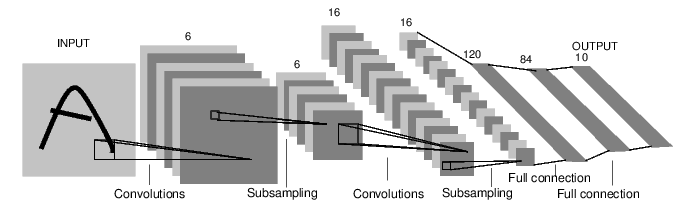
It is important to understand what a facial recognition task entails. The generalized architecture of facial recognition architecture is as follows:

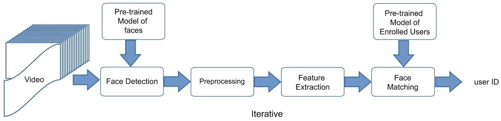
Whatever the input you provide for a face detection model, there is a backend facial detector model. In DeepFace library, the available backend detectors are: opencv, dlib, mtcnn, retinaface, mediapipe, yolov8, yunet, and others. As mentioned in the previous tech note, yolov8 and the likes are object detection models. The video or image is imputed and the step of detection is very important because the face should be well-bounded so no facial feature is lost. This step in the workflow is essential because it includes face alignment too. Face alignment is important because what later models do in the recognition architecture is to extract features using mathematical relationships. Therefore, alignment is crucial and this is supported by the fact that it can increase accuracy by up to 1% as the DeepFace library documentation mentions. Alignment is, hence, part of the preprocessing stage. Thus we can say that we have a number of state-of-the-art face detectors available to us to fulfill the two first steps of the facial recognition architecture (i.e., face detection and preprocessing).

For feature extraction and all its consequent applications (i.e facial embedding, recognition, etc) the available models are: Facenet, Facenet512, ArcFace, VGGFace, SFace, OpenFace, Dlib and others. Their performance on LFW dataset are as follows as mentioned in the DeepFace library documentation:

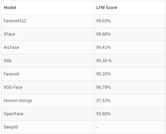
Human beings scored an accuracy of 97.53, outperformed by Facenet512, SFace, ArcFace, Dlib, Facenet, and VGGFace. These are the newest models available mostly depending on deep convolutional neural networks storing the relationships between facial features and storing them in facial embedding vectors for later comparison, recognition, and finally labeling.

After this step of feature extraction, we have the distance metric responsible for quantifying similarity. The options for similarity measures are: cosine similarity, euclidean distance, and l2 normalized euclidean distance. Theoretically speaking, the last measure provides a more stable and less volatile measure of similarity based on experiments. However, the default measure used by DeepFace is cosine similarity. Based on a certain threshold for each measure, a decision is made whether or not two faces are of the same person or not.

Getting Technical: Architecture Optimization

This tripartite architecture allows a great deal of flexibility in terms of the customization of the configuration of the facial recognition architecture. The customization should be directed by the purpose behind the task in the first place. In our case, it is to detect fraudulent assistance requests, i.e. a beneficiary who tries to receive assistance more than the assigned number of times. As with any classification problem, we have two types of errors: False Positives and False Negatives. A false positive in our case, is when somebody is classified as a duplicate (i.e. their face exists in the database of images of beneficiaries indicating that they took assistance before) while this is not truly a duplicate. False negatives, on the other hand, indicate that a beneficiary was classified as not a duplicate while in fact he/she was a duplicate.

It is important for us, as Data Scientists, to identify which error is more critical so that we configure the architecture in a way that minimizes this error. Obviously the purpose of WFP’s field work is to provide assistance for those in need, thus it is fatal for WFP to claim that a beneficiary took food before while in fact they didn’t. Hence, we want to penalize this error and find the best configuration of the given models for each task in the facial recognition architecture. Here, the task at hand is very similar to hyperparametric optimization for Neural Networks and other machine learning models, however it is not the weights and parameters of a model we are trying to optimize but the configuration of a whole architecture which contains two models, and a distance/similarity measure.

In hyperparametric optimization, you have three main elements:

1. Hyperparameter space

2. Objective function

3. Optimization algorithm

4. Testing data

The first is basically all the combinations of the parameters you want to change for optimizing the model’s performance. The objective function is the function you decide with on which is the best set of parameters, i.e. the best set of parameters are identified such that they maximize or minimize the objective function. The optimization algorithm is how this optimal solution is found, the most known ones are:

1. Bayesian Optimization

2. Random Search

3. Grid Search

Lastly, one would need a set of images on which the performance of the model will be calculated given a certain combination of parameters.

To avoid getting in messy details about each optimization algorithm, each one of them will be described briefly:

1. Bayesian Optimization: is a sequential design strategy for global optimization of black-box functions that does not assume any functional forms.

2. Random Search: is a family of numerical optimization methods that do not require the gradient of the problem to be optimized.

3. Grid Search: is a process that searches exhaustively through a manually specified subset of the hyperparameter space of the targeted algorithm.

Grid search is the easiest one of them conceptually because it is a brute force algorithm going through all possible combinations. Since we don’t have a huge number of combinations available and since we want to know how each one performed, grid search was chosen for this task.

Now we need three more elements for us to be able to perform the architectural optimization we are trying to achieve. First of all, the equivalent of hyperparametric space, which will be in our case all the combinations of models available. Because of some technical issues with some backend detectors and some feature extraction models and since the difference between euclidean and l2-euclidean distances was minimal, our space was as follows:

1. Models: Facenet512, Facenet, OpenFace, ArcFace, and SFace

2. Backend Detectors: retinaface, mtcnn, mediapipe, and dlib

3. Distance Metrics: cosine similarity and euclidean distance.

This makes for 40 combinations total. Followingly, we need a testing dataset. We compiled some difficult pictures to detect in this dataset. Some examples are as follows:

Those three sets of images represent three challenges respectively: different people but look very alike, same person but different age, same person different facial expression. The dataset is basically divided into these classes where for each case there are sets of images that pose one of those challenges.

Now that we have the experimentation space, the optimization algorithm, and the dataset, we need an objective function. Our objective function should be minimizing the number of false positives because this is the worst error while maintaining a low rate of false negatives as well. For this end, I chose the F-ꞵ score which is a variation of the F-1 score (which the harmonic mean of precision and recall).  F-ꞵ score allows us to put more weight on the precision because high precision means less false positives, while still taking into account the value of the recall which is directly proportional to the number of false negatives. The equation for the F-ꞵ score such that more weight is directed to precision is as follows:

In our case, we used ꞵ=2. To see how this score works, assume precision to be 0.5 (i.e. a low precision) and a high recall like 0.9 for example. Now the F-2 score will equal 0.55. Now if precision is 0.9 and recall is 0.5, F-2 score will be 0.78. This indicates that precision will always be more important and skew the F-2 towards it. Now after 5+ hours of runtime, the best architecture configuration with a staggering F-2 score of 1, was identified.

An F-2 score of 1, means that precision and recall were both 1, indicating that the model had no mistakes. This is surprising given that Facenet512 was said to be the best performing model and retinaface was said to be the best backend detector. However, our combination was different!

Outperforming Humans

What did it take for face detection libraries to outperform humans after this architectural optimization we conducted? Why this combination though? The answer is difficult but what we could do is explain briefly what both of them provide and how they both could be a good fit for each other along with the cosine similarity metric.

What makes ArcFace for example stand out from most face recognition models is the fact that it uses Additive Angular Margin Loss while others use Softmax. According to an implementation of ArcFace from scratch on kaggle, ArcFace works as follows:

1. Normalize the embeddings and weights

2. Calculate the dot products

3. Calculate the angles with arccos

4. Add a constant factor m to the angle corresponding to the ground truth label

5. Turn angles back to cosines

6. Use cross entropy on the new cosine values to calculate loss

Thus, it makes sense that cosine similarity would be the best fit for this model. Anyhow, ArcFace provides more compact clusters compared to softmax as shown below:

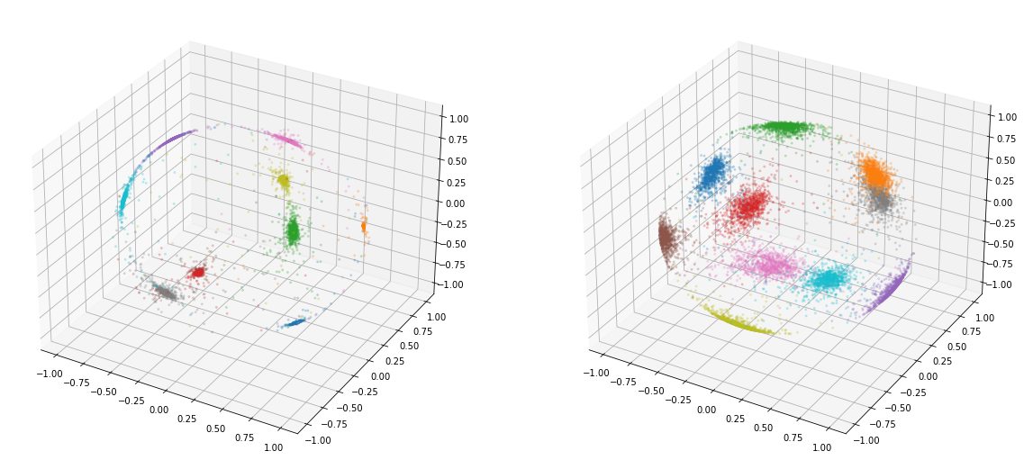
ArcLoss // Softmax

Dlib, on the other hand, uses the HOG algorithm or the Histogram of Oriented Gradients. According to this article, the HOG algorithm functions as follows:

It uses five filters for each face:

1. Frontal face

2. Right side turned face

3. Left side turned face

4. The frontal face but rotated right

5. The frontal face but rotated left

This means that the detection would be 3 dimensional. All things considered, it makes sense that ArcFace provides the best scores with cosine similarity because the embedding itself is angular. ArcFace on its own is expected to over perform given how compact its feature extraction clusters are. When it comes to the relationship between the model and backend detector it is a bit unclear.

What’s Next

The next steps should be fixing or identifying the technical issues which forced us to decrease our experimental space to only 40 combinations. We could then fix them and maybe find new  potential for the DeepFace library configuration. It is also important to overcome dependency on DeepFace library and implement the algorithms locally to allow for fine-tuning, training, and more customizability in general. Generally, these are improvements that are directed at scaling-up this solution but what remains as the most important next step is testing this model on various amounts of data to locate its weak points and help improve the model so as to overcome them if possible.